Training the lattice
In this blog I am presenting a new model for Quantum Mechanics based on local-realistic rules for ensemble of particles. A first version of the model has been published in this journal; an extended version in this preprint.
In a previous post, I have shown that the direct simulation of the rules of motion, even for a relatively simple quantum scenario such as a two-slit experiment, can take an unpractically long computing time. In fact, the dynamics of the lattice and particle bosons involved may take a large number of iterations before they converge to the values from which the stanbdard QM behavior emerges.
This post discusses a first method to accelerate the simulations. This method consists in assuming that all lattice boson momenta have already converged to their steady-state values. This normally happens only after a large number of particle emissions of the same ensemble has been simulated, so that many particles have visited each lattice node. Here we assume that this process has already happened, that is, that the lattice is already trained after a large number of non-simulated emissions.
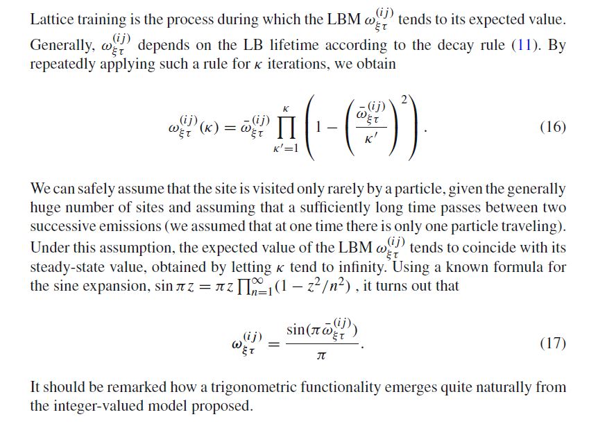
To evaluate the steady-state value of Lattice Boson Momenta, we take some extracts from the journal publication:
 where the rule (11) mentioned has been discussed in this post, and
 where rule (8) is the initialization rule of the LBM also discussed in that post. We forget for the moment the role played by the source phase ε, which will be discussed in a future post.
In summary, and with the nomenclature used elsewhere in this blog, the lattice training is completed when the LBM take the values
}=\frac{\sin(\pi|\ell-\lambda|x/t)}{\pi} "\omega_{xt}^{(\ell\lambda)}=\frac{\sin(\pi|\ell-\lambda|x/t)}{\pi}")
We can observe lattice training by analysing the results of a simulation performed with this code. The figure below compares the values of ωxt (blue crosses) with its steady state values (orange marks) - given by the right-hand side of the previous equation -, for all x comprised between -Nt and Nt. The simulation ran with Nt = 300, Np = 300000, Ns = 2, xs = [-1,1], Ps = [0.5,0.5].
 As the figure shows, 300000 emissions of 300 iterations each are not sufficient to see the convergence of the LBM to their steady-state values. In fact, when Nt is too small, particles might arrive, with non-negligible probability, at nodes that are substantially different from the expected arrival node. When this is the case, their momentum propensity at node arrival differs from the ratio x/t. Consequently, the initial LBM do not necessarily coincide with the expected value shown in the paper's equation (18) displayed above and the convergence of the LBM to the theoretical value is prevented. On the other hand, in order to simulate large values of Nt, a large number of emissions (large Np) is necessary, otherwise several nodes would be visited by too few or no particles. The combination of large Nt and large Np makes the simulation unpractical (large size of the arrays involved, large number of iterations).
However, the good trend is clearly visible already in the figure above, which is ecouraging. In a next post, we shall present an accelerated code for simulation of particle emissions that assumes an already trained lattice.

This post discusses a first method to accelerate the simulations. This method consists in assuming that all lattice boson momenta have already converged to their steady-state values. This normally happens only after a large number of particle emissions of the same ensemble has been simulated, so that many particles have visited each lattice node. Here we assume that this process has already happened, that is, that the lattice is already trained after a large number of non-simulated emissions.
To evaluate the steady-state value of Lattice Boson Momenta, we take some extracts from the journal publication:

In summary, and with the nomenclature used elsewhere in this blog, the lattice training is completed when the LBM take the values
We can observe lattice training by analysing the results of a simulation performed with this code. The figure below compares the values of ωxt (blue crosses) with its steady state values (orange marks) - given by the right-hand side of the previous equation -, for all x comprised between -Nt and Nt. The simulation ran with Nt = 300, Np = 300000, Ns = 2, xs = [-1,1], Ps = [0.5,0.5].

However, the good trend is clearly visible already in the figure above, which is ecouraging. In a next post, we shall present an accelerated code for simulation of particle emissions that assumes an already trained lattice.


Comments
Post a Comment