Quantum forces in a nutshell

After having described in the previous posts the motion of an ensemble of particles emitted at the same, perfectly localized in space, source, it is time to turn our attention to the emergence of quantum forces, which ultimately leads to the description of phenomena such as quantum superposition and the related interference.

In this post, we shall discuss about the famous double-slit experiment and see how it is treated in the proposed model. In future posts, we will generalize the concepts introduced here.

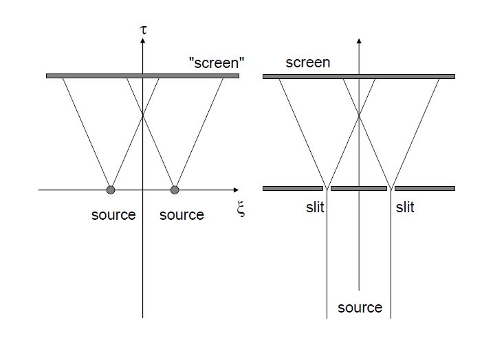
Consider a simplified, 1D version of a double-slit apparatus. where similar particles are emitted at a certain rate from either of two sources placed at positions x₀ = ±δ. Emitted particles have a constant speed along the perpendicular y direction, but a random initial speed along the x direction. At a certain distance from the sources along the y axis, a backstop is placed and particle arrivals are detected. Given the constancy of the y-axis velocity, will assume that all particle reach the backstop after the same time T. We will thus consider only motion along the x direction and we are interested in evaluating the frequency of arrivals P(x) at the backstop.

The Quantum Mechanical result is known to be (in lattice units):

(1)

where P₁ and P₂ are the probabilities that a particles is emitted from source 1 (say, -δ), resp., 2 (+δ), and P₁+P₂ =1 holds. Obviously, the integral of the QM probability at the backstop, that is, between x = -T and x = +T, is one. The proposed model is alble to retrieve this result from a fundamental mechanism (that is local and realistic) and not by adding the probability amplitudes and squaring the modulus per the Bohm rule. Here it is how it does.

The first key idea is that the momentum propensity V of the various particles emitted does not coincide anymore with their source momentum v₀ that is randomly attributed. In fact, it turns out that in this double-slit situation the momentum propensity tends to a value such that

(2)

We shall see later how this is possible. In any case, since v₀ is a stochastic variable, so is V. Its pdf can be easily calculated by applying again the properties of probability density functions under changes of variable, which yields

Now, the average position at the backstop at time T is given by ⟨x⟩ = x₀+VT. By applying again the "chain rule" of probability densities above, we obtain the sought form of P(x), for times large enough that δ can be considered small (a more rigorous derivation is postponed to future posts).

So in a nutshell the quantum superposition is the result of the mechanism for which the momentum propensity diverges from its initial value, the source momentum, and converges to a different value, which still depends on v₀. Actually, the dependency between v₀ and V is monotonic and, moreover, ensures that, for v₀ = ±1, also V = ±1 holds. This fact is very important since it ensures that the momentum propensity never becomes superluminar.

We illustrate now the proposed mechanism leading to the momentum propensity drift. Continuously during their flight, the various particles leave to the lattice nodes a footprint of their passage, consisting of the distance ℓ they have covered so far. At node x, particles emitted at source 1 leave a footprint 𝛿 + x, while for particles emitted at source 2, the footprint is −𝛿 + x. Moreover, each particle is capable to sense the footprint 𝜆 left by the particle that has previously visited that lattice node, that is, crossed its current position at the same flight time.

When a particle arrives at a node, there are two possibilities. The first case is when 𝜆⁡ is equal to ℓ. This happens when the flying particle leaves from source 1 and finds the footprint of a previous particle equally emitted from 1, or when the flying particle is from source 2 and finds the footprint of a previous particle equally emitted from 2. This circumstance, which we may label “a”, has thus a probability P_a = P₁²+P₂² to happen. The second case is when 𝜆 is different from ℓ. This happens when a flying particle from 1 finds the footprint of a particle emitted from 2, or vice versa. Thus, in this circumstance, |𝜆 − ℓ| = 2𝛿. This event “b” has probability P_b = 2P₁P₂. Note that P_a+P_b = 1, as it should be.
When an event “b” occurs, a pair of entities (called “bosons” in the following) is created, one of which is attached to the flying particle and the other to the footprint. The newly created bosons replace possibly existing bosons that were already attached to the particle or to the footprint, respectively (resulting from a previous event “b”).

Both bosons carry a momentum contribution. The momentum of the new particle boson v_b equals the previous momentum of the footprint boson, 𝜔, divided by the difference |𝜆 − ℓ|, that is, 2𝛿. On the other hand, the new footprint momentum equals the momentum propensity of the visiting particle multiplied by 2𝛿. In other terms, there is an exchange of momentum information between the particle and the footprint.

Once created, the footprint momentum decays with a particular law that is approximately ~ exp(1/
time), unless the footprint is replaced by a new one left by another particle (another event “b”).
However, the expected lifetime of a footprint is very long, since only one footprint is visited at each
time by the currently flying particle, and particles are emitted at a finite rate. The footprint momentum has thus enough time to converge to a steady-state value that, as it will be shown in a future post, is

 

where the barred omega is the momentum at the footprint creation that, as anticipated above, is proportional to the momentum propensity of the particle that left the footprint.

As for the momentum of the flying particle’s boson v_b, it is reset to the value sin(2𝜋𝛿V) /𝜋𝛿 (see
above) at each event “b”. Otherwise, as long as an event “a” occurs, v_b decays with a particular law
that is approximately ~1/√time. It will be shown in a future post that the average value
taken by particle boson momentum as a consequence of this rise-and-decay behaviour is

as it clearly depends on the relative probability of the events “a” and “b”.

The last rule is that momentum propensity of the particle equals by the difference between its source momentum and the momentum contributed by the boson, V = v₀ − v_b, which ultimately yields the steady-state relation (2) above and thus to the sought pdf (1).